Mathematical Modeling Slideshow
Introduction to Mathematical Modeling
Those who are smart can be lazy, but those who are lazy cannot be smart."
-Professor Thomasey
A mathematical model, by definition, is "a description of a system using mathematical knowledge and language". Mathematical modeling can be applied to many different things, including biology, chemistry, and engineering. During their four weeks at Governor's School for Mathematics, Science, and Technology, Professor Thomasey's students learned the basics of mathematical modeling, including programming with the Maple mathematics program, problem-solving, and the application of differential equations.
Feel free to browse around to find out more about mathematical modeling at Governor's School and the students' work during their four weeks.
Feel free to browse around to find out more about mathematical modeling at Governor's School and the students' work during their four weeks.
Proof for Pythagoras
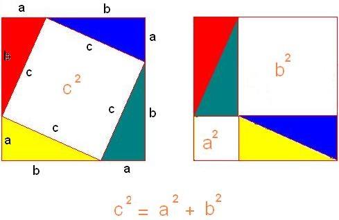
We all use Pythagorean Theorem in simple mathematics. With the lengths of two sides of a triangle, we are able, through this theorem, to solve for the third unknown side. Here is a geometric proof of this theorem. In this diagram, “a,” “b,” and “c” label the short and long legs and the hypotenuse of each triangle. Using the formulas for the area of a triangle and square, it is shown that a^2 + b^2 = c^2 as the Greek mathematician proposed.
Euclidean Algorithm
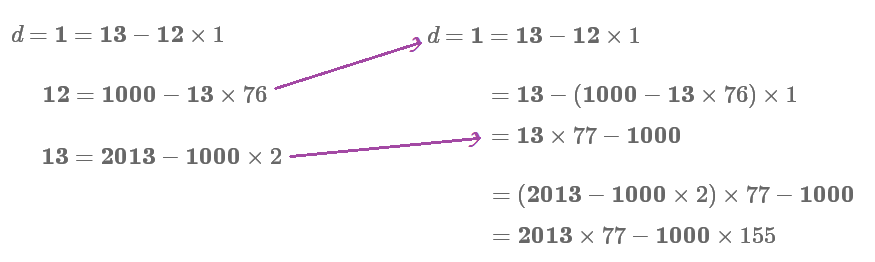
The Euclidean algorithm is a process to determine the greatest common denominator of any two pairs of numbers. The two numbers can be defined as the variables a and b, while a>b. The process states to use the equation a = qb + r and replace a with the next b and to replace b with the next r until the value of r reaches 0. The variable r defines the remainder left over when b is multiplied with the closest number q to reach a. When r = 0, the number for b is the greatest common denominator.
Proving by Mathematical Induction
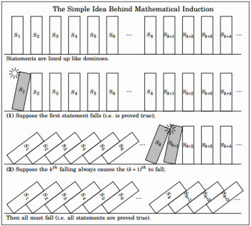
Mathematical induction is a method of mathematical proof typically used to establish a given statement for all natural numbers. It is done in two steps. The first step is to prove the given statement for the first natural number. The second step is to prove that the given statement for any one natural number implies the given statement for the next natural number. From these two steps, mathematical induction is the rule from which we infer that the given statement is established for all natural numbers.
Modeling Population Growth
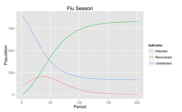
Professor Thomasey's students began to model susceptible/infected populations, a model where there are two groups, healthy population and infected/sick populations. People can be born into either the healthy population or the infected population. People can also become infected from the healthy/susceptible group, therefore increasing the population of the infected. Both groups also have a mortality rate so they populations won’t exponentially increase. They also tried to keep the model realistic by having assumptions that could be applicable in the real world, for example, keeping the birth rate higher than the death rate and having the death rate of the infected population higher than the death rate of the healthy population. When they were modeling, they had several parameters, the birth rates of both groups, the death rates of both groups, and the interaction rate between the two groups (the rate at which the healthy becomes infected).
Going Deeper into Populations: The Lotka - Volterra Model
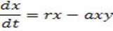
The Lotka-Volterra model looks at the oscillating relationship between predator and prey populations. In the first equation, the “rx” term is the population growth for the prey. Similarly, “-my” details the death rate for the predator. The “axy” and “bxy” terms are the interactions between prey and predator. There are several assumptions involved in this model:
1. r > a, otherwise “x” would die out. Must be a fairly large number in order to maintain prey population.
2. a b since population gains or losses are usually not 1 for 1.
3. b > m, otherwise “y” would die out.
The Lotka-Volterra Model is crucial in the examination of population growth and decay and is largely used to demonstrate the predator - prey model.
Fun with Matrices!
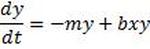
In mathematics, a matrix is a rectangular array of numbers, symbols, or expressions, arranged in rows and columns. They are commonly used for the representation of large groups of numbers and to compute operations on those numbers. We learned about many things involving matrices, including multiplication, the identity matrix, and the determinant of a matrix.
La Tierra de Eigen - The Power of Eigenvalues
Eigenvalues (only for square matrices) are scalars λ such that AX=λ x, where x is an eigenvector.
Eigenvalues tell what type of solutions will occur from differential equations.
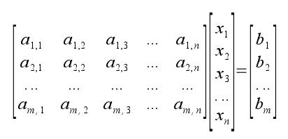
Types of solutions
Case 1: λ1˂0, λ2˂0
Result: attractor, steady state solution. Everything tends toward the solution
Case 2: λ1˃0, λ2˂0 or λ1˂0, λ2˃0
Result: saddle, somewhat stable solution. Values will either be attracted to or repelled by the solution, depending on the initial condition.
Case 3: λ1˃0, λ2˃0
Result: repeller, the system can never reach the solution. It could also result in an oscillating, unstable spiral, where it is unknown how the system will react.
Eigenvalues tell what type of solutions will occur from differential equations.
Types of solutions
Case 1: λ1˂0, λ2˂0
Result: attractor, steady state solution. Everything tends toward the solution
Case 2: λ1˃0, λ2˂0 or λ1˂0, λ2˃0
Result: saddle, somewhat stable solution. Values will either be attracted to or repelled by the solution, depending on the initial condition.
Case 3: λ1˃0, λ2˃0
Result: repeller, the system can never reach the solution. It could also result in an oscillating, unstable spiral, where it is unknown how the system will react.
